This article first briefly introduces the basic principles of FM, a general digital demodulation scheme, points out the existence of the FM demodulation threshold, and gives the simulation results; then discusses the noise problem in detail, pointing out the relationship between the autocorrelation characteristics of noise and the channel filter And according to these properties of noise, a new digital demodulation scheme is proposed, and finally the actual simulation results of the new scheme.
The basic principle of FM
FM is to modulate the signal to the frequency parameter of the carrier. The difference between the instantaneous frequency and the average frequency is the signal. The expression is as follows:

The following figure is the time domain and frequency domain waveforms of the FM signal generated by ADS. From the time domain waveform, the constant envelope characteristics of FM and the characteristics of the instantaneous frequency change with time can be clearly seen. The FM carrier frequency generated here is 200KHz, mono, and the modulated signal is
5KHz frequency, 65KHz modulation, no pre-emphasis is considered.

Figure 1: Frequency domain waveform of FM signal

TIme, msec
Figure 2: Time domain waveform of FM signal
Simple digital demodulation and threshold effect of FM uses digital methods to demodulate the FM signal. In principle, it is to calculate the instantaneous frequency. The instantaneous frequency is the derivative of the phase. In the digital, the derivative is replaced by the first-order difference. The following is a simple FM digital solution Adjust the block diagram:

Using the above simple demodulation method, we adjust the input signal-to-noise ratio and look at the change of the output signal-to-noise ratio, we can clearly see the existence of the threshold. The following is the simulation data and curve graph:
Table 1: Simple digital demodulation input SNR and output SNR relationship, where the FM modulation is 22K, mono
SNR in 5 6 7 8 9 10 11 12 13 18 23 28
SNRout 9.5 12.8 16.5 20.2 23.4 24.5 25.6 26.6 27.6 32.7 37.7 42.6

Figure 4: Schematic diagram of FM demodulation. Note that the above does not consider de-emphasis to improve the signal-to-noise ratio. The noise is to consider the noise in the 1.5k ~ 15K bandwidth. The input noise is the noise within the filter bandwidth, and the channel filter is calculated at 70K. It is obvious from the above curve that the input signal to noise ratio
Below 9dB, the output SNR and input SNR are no longer linear. The input signal has a corner at 9dB, which is called the demodulation threshold of this demodulation scheme.
From the IQ plane, it is easier to understand the existence of the demodulation threshold. As shown in the figure below, when the signal-to-noise ratio is low, the noise vector is sometimes larger than the signal vector, causing a phase change of 180 degrees, which causes a rapid increase in noise, which forms a threshold. Generally, the weak signal is limited by the noise figure of the receiver, and the noise reflected by the noise figure conforms to the Gaussian distribution. From the function of the Gaussian distribution, there are very few cases where the standard deviation exceeds 3 times, that is, when the SNR is greater than 20log (3), There is rarely a 180 degree flip, so 20log (3) becomes the demodulation threshold of FM. 20log (3) = 9.5dB, which is in good agreement with the above simulation curve.
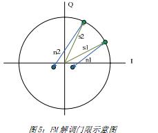
Figure 5: Schematic diagram of the FM demodulation threshold. Noise autocorrelation characteristics and noise prediction. The noise limited by the receiver to receive weak signals is generally receiver thermal noise, current noise, etc. These noises can be regarded as white noise for our signal bandwidth This also means that the noise is not related before and after. Fortunately, the receiving channel has a channel selection filter. In the digital decision, the noise is related before and after the noise. Because this correlation is caused by the receiving channel filter, the noise The autocorrelation function of is equal to the autocorrelation function of the impulse response of the filter, and its formula is as follows:
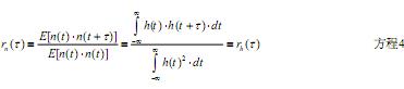 In the above formula, h (t) is the time-domain impulse response of the channel filter. Because the channel filter of a general receiver is fixed, the autocorrelation characteristic of noise is determined.
If the noise voltage at time t1 is n1 and the noise voltage at t2 is n2, what is the noise voltage at t3?
Here we can make a decomposition of the noise voltage n3 at time t3, and separate the relevant part and the unrelated part, as follows:
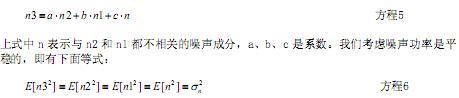
Based on the noise-related characteristics discussed earlier, we can obtain the following equations:
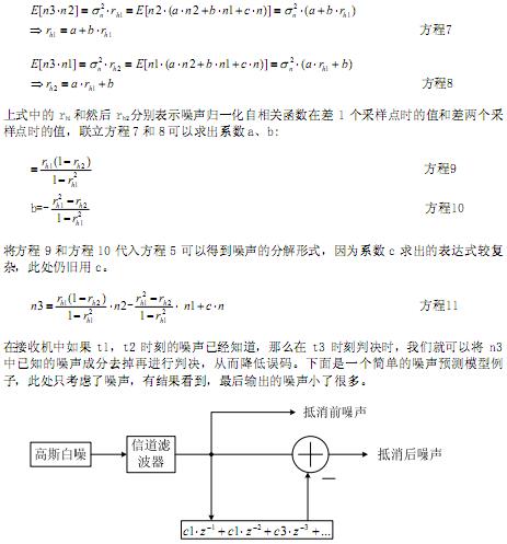
Figure 6: Schematic diagram of noise prediction and cancellation c1, c2, c3, ... in the above figure are parameters related to the channel filter. If there is no channel filter in the above figure, the noise is not related before and after, and these coefficients are all 0. The previous equations 5 to 10 have already discussed how to calculate the coefficients of the second-order case.
I won't repeat them here. The following is the simulation results using ADS, where the filter bandwidth is 70K, and the digital clock uses
At 500K, the noise prediction model is second-order, because the analysis shows that the noise difference of 3 clocks is basically irrelevant.
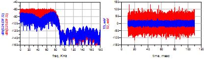
Figure 7: Schematic diagram of noise cancellation. In the above figure, red is the frequency and time domain noise waveforms before cancellation, and blue is the frequency and time domain noise waveforms after cancellation. Here we can see that the noise power is suppressed a lot. The use of noise cancellation has great benefits, but the premise is that the noise component must be found relatively accurately, that is, the signal component in the sampling point. Signal and noise are combined. If you want to separate them, you need a decision process. For digital communications, this decision is often obvious, such as QPSK
Demodulation, when judging, just look at (I, Q), if it falls in the first quadrant, we judge it as (1,1), and in the second quadrant, we judge it as (-1,1 ), The vector from the ideal constellation point to the actual IQ is the noise component, as shown in the following figure:
 FM signal decision and noise cancellation Through the above discussion, we can sort out such a receiver model, as shown below:

The noise prediction and decision in digital communication have been discussed earlier. How should we decide for FM signal? The FM signal does not have the best decision time often found in digital communication, but FM has a very obvious feature. Ideal FM is a constant envelope. We can make a decision based on this feature. Obviously this decision cannot completely distinguish between noise and noise. Signal, because the tangential component of noise cannot be separated from the signal, however, this kind of decision can still solve the problem of FM demodulation threshold better. The following figure makes it easier to understand this judgment and understand its limitations:
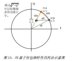
Figure 10: Schematic diagram of FM decision based on constant envelope characteristics. From the above figure, the ideal noise component is n1, and we only found the normal noise component n1r, and n1t can not be identified. Where. Using this decision principle, we built the following simulation circuit diagram and made a simulation analysis:
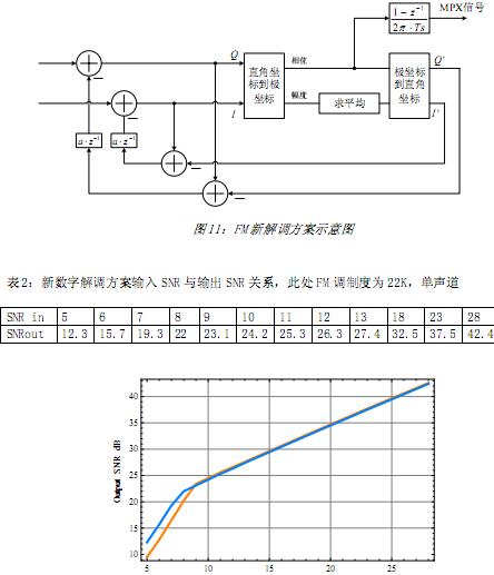
Figure 12: Comparison of the performance of the new and old digital demodulation schemes The blue figure above is the performance curve of the new demodulation scheme. The comparison shows that the new demodulation scheme can reduce the demodulation threshold by 1dB. In weak field reception, the output signal-to-noise ratio is improved 3dB.
Screw Terminal Connector,Pcb Screw Terminal,Screw Terminal Block Connector,Screw Type Terminal Blocks
Cixi Xinke Electronic Technology Co., Ltd. , https://www.cxxinke.com