TensorFlow learning to build a neural network add layer
1. Create a Neural Network Layer
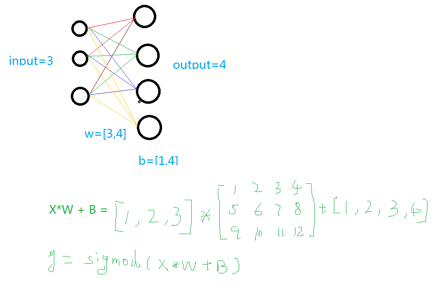
To build a neural network, you need to define the input value, input size, output size, and the activation function. If you're familiar with neural networks, the following image should make sense. If not, feel free to check out my other blog post for more details (http://).
The code for creating a layer is as follows:
def add_layer(inputs, in_size, out_size, activate=None):
Weights = tf.Variable(tf.random_normal([in_size, out_size])) # Random initialization
Baises = tf.Variable(tf.zeros([1, out_size]) + 0.1) # Better to use fixed values than zero
y = tf.matmul(inputs, Weights) + Baises
if activate:
y = activate(y)
return y
2. Train a Quadratic Function
Let's start by importing TensorFlow and NumPy:
import tensorflow as tf
import numpy as np
Then we define the add_layer function again, which we already have from before.
Next, we generate some sample data that follows a quadratic function with added noise:
X_data = np.linspace(-1, 1, 300, dtype=np.float32)[:, np.newaxis]
Noise = np.random.normal(0, 0.05, X_data.shape).astype(np.float32)
Y_data = np.square(X_data) - 0.5 + Noise
We then create placeholders for the inputs and labels:
xs = tf.placeholder(tf.float32, [None, 1])
ys = tf.placeholder(tf.float32, [None, 1])
Now, we build our neural network:
L1 = add_layer(xs, 1, 10, activate=tf.nn.relu)
Prediction = add_layer(L1, 10, 1, activate=None)
Define the loss function and optimizer:
Loss = tf.reduce_mean(tf.reduce_sum(tf.square(ys - prediction), reduction_indices=[1]))
Train_step = tf.train.GradientDescentOptimizer(0.1).minimize(loss)
Finally, we initialize the session and run the training loop:
sess = tf.Session()
sess.run(tf.global_variables_initializer())
for i in range(1000):
sess.run(train_step, feed_dict={xs: X_data, ys: Y_data})
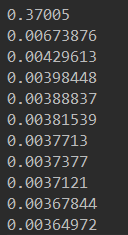
if i % 50 == 0:
print(sess.run(loss, feed_dict={xs: X_data, ys: Y_data}))
3. Dynamic Visualization of Training Process
This section explains how to visualize the training process dynamically. We use Matplotlib for real-time plotting.
Import necessary libraries:
import matplotlib.pyplot as plt
We then create a plot and display it:
fig = plt.figure('show_data')
ax = fig.add_subplot(111)
ax.scatter(X_data, Y_data)
plt.ion()
plt.show()
During training, we update the plot every 50 steps:
if i % 50 == 0:
try:
ax.lines.remove(lines[0])
except Exception:
pass
prediction_value = sess.run(prediction, feed_dict={xs: X_data})
lines = ax.plot(X_data, prediction_value, 'r', lw=3)
print(sess.run(loss, feed_dict={xs: X_data, ys: Y_data}))
plt.pause(2)
While True:
plt.pause(0.01)

4. Overview of TensorBoard Visualization
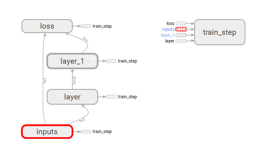
TensorBoard provides a powerful way to visualize the structure of your model. To use it:
A. Use `tf.name_scope` to organize your graph into different sections.
B. Write the graph to a file using `tf.summary.FileWriter`.
C. Run TensorBoard with the command: `tensorboard --logdir=test`.
Make sure to navigate to the correct directory where your log files are stored before running the command.
5. Localized Display with TensorBoard
You can also visualize specific aspects of your model locally using TensorBoard:
A. Use `tf.summary.histogram` to display weight distributions.

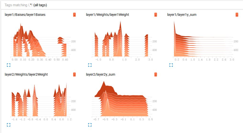
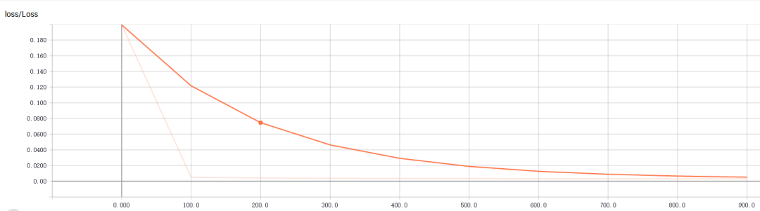
B. Use `tf.summary.scalar` to track the loss over time, which is crucial for evaluating training progress.
C. Initialize and run the summary operations:
merge = tf.summary.merge_all()
writer = tf.summary.FileWriter("G:/test/", graph=sess.graph)
result = sess.run(merge, feed_dict={xs: X_data, ys: Y_data})
writer.add_summary(result, i)
Here’s the complete code for a more detailed visualization:
import tensorflow as tf
import numpy as np
import matplotlib.pyplot as plt
def add_layer(inputs, in_size, out_size, n_layer=1, activate=None):
layer_name = "layer" + str(n_layer)
with tf.name_scope(layer_name):
with tf.name_scope("Weights"):
Weights = tf.Variable(tf.random_normal([in_size, out_size]), name="W")
tf.summary.histogram(layer_name + "Weight", Weights)
with tf.name_scope("Baises"):
Baises = tf.Variable(tf.zeros([1, out_size]) + 0.1, name="B")
tf.summary.histogram(layer_name + "Baises", Baises)
y = tf.matmul(inputs, Weights) + Baises
if activate:
y = activate(y)
tf.summary.histogram(layer_name + "y_sum", y)
return y
if __name__ == '__main__':
X_data = np.linspace(-1, 1, 300, dtype=np.float32)[:, np.newaxis]
Noise = np.random.normal(0, 0.05, X_data.shape).astype(np.float32)
Y_data = np.square(X_data) - 0.5 + Noise
fig = plt.figure('show_data')
ax = fig.add_subplot(111)
ax.scatter(X_data, Y_data)
plt.ion()
plt.show()
with tf.name_scope("inputs"):
xs = tf.placeholder(tf.float32, [None, 1], name="x_data")
ys = tf.placeholder(tf.float32, [None, 1], name="y_data")
L1 = add_layer(xs, 1, 10, n_layer=1, activate=tf.nn.relu)
Prediction = add_layer(L1, 10, 1, n_layer=2, activate=None)
with tf.name_scope("loss"):
Loss = tf.reduce_mean(tf.reduce_sum(tf.square(ys - Prediction), reduction_indices=[1]))
tf.summary.scalar("Loss", Loss)
with tf.name_scope("train_step"):
Train_step = tf.train.GradientDescentOptimizer(0.1).minimize(Loss)
sess = tf.Session()
merge = tf.summary.merge_all()
writer = tf.summary.FileWriter("G:/test/", graph=sess.graph)
sess.run(tf.global_variables_initializer())
for i in range(1000):
sess.run(Train_step, feed_dict={xs: X_data, ys: Y_data})
if i % 100 == 0:
result = sess.run(merge, feed_dict={xs: X_data, ys: Y_data})
writer.add_summary(result, i)
Usb3.2 20Gbps Data Cable,Usb 3.2 Type-C,Usb3.2 Type-C Charging Data Cable,High-Speed Usb 3.2 Type-C
Dongguan Pinji Electronic Technology Limited , https://www.iquaxusb4cable.com